Introduction to Actuarial Data Science
Actuarial Data Science - Open Learning Resource
With the rise of AI and big data, every firm has effectively become a data-driven enterprise. Whether it is supermarkets, hairdressers, restaurants, or dentists, businesses of all types are collecting data on customer behaviour and engagement. We are living in a data-driven era, where data has become one of the most valuable assets for businesses. However, possessing data alone does not automatically translate into insights or business value. It is crucial to apply appropriate data science techniques to extract meaningful insights and communicate those findings effectively to stakeholders.
There are many textbooks available today that cover data science, statistical methods, and machine learning techniques. What does this Open Learning Resource (OLR) offer that is different? While many excellent data science textbooks exist, they often focus on individual techniques or models without addressing the entire problem-solving process in a business setting. In contrast, this OLR aims to equip readers with the skills to solve data problems in real-world business environments. It guides readers through the complete process: from asking the right questions and performing exploratory data analysis to modeling, interpreting results, communicating findings, and considering ethical implications.
The aim of this learning material is aligned with the Australian Actuaries Institute’s Part II Data Science Principles syllabus.
“The Data Science Principles aim to extend students’ knowledge of modern analytical tools and techniques beyond those introduced in the Foundation Program subjects and to teach students how to apply this knowledge in real-life business settings”
— Actuaries Institute, Data Science Principles syllabus
Data science is an interdisciplinary field that covers many areas of knowledge, including but not limited to statistics, machine learning, databases, optimization, algorithms, programming, and domain knowledge in a business setting. This book mainly focuses on applying the data analysis cycle with statistical machine learning techniques to address actuarial applications, referred to as Actuarial Data Science. The techniques and concepts introduced in this book can be applied more broadly to other business problems. Therefore, this book can also be used as a textbook for solving general business data problems.
It is often argued that data science is a discipline rooted in science and engineering, with a vast arsenal of quantitative tools. However, it is important to recognise that data science is also an art (Peng and Matsui 2015). While a wide range of analytical techniques—from linear regression to classification trees and deep learning—have been codified into software packages, the role of the data scientist extends far beyond selecting and running algorithms. Effective data science involves making numerous judgment calls throughout the problem-solving process: choosing appropriate tools for specific tasks, interpreting results, communicating findings clearly to stakeholders, and embedding ethical and regulatory considerations into each decision. These nuanced aspects of data science—judgment, interpretation, and communication—remain, at least for now, beyond the capabilities of machines.
Data Science Lifecycle (DSL)
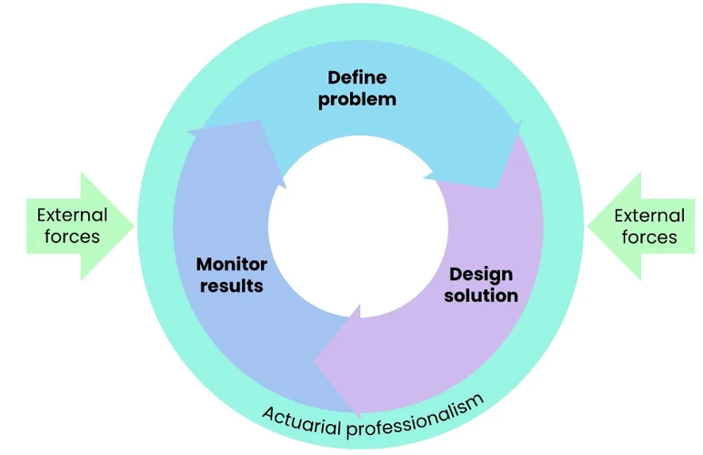
Actuaries apply the Actuarial Control Cycle (ACC), as shown in Figure 1 for problem solving.
Figure 1 is adapted from the Actuaries Institute, based on Bellis et al. (2010).
In a similar spirit, we introduce the Data Science Lifecycle (DSL) as a practical methodology for tackling data-driven problems. While rooted in the principles of the ACC, the DSL reflects the unique, iterative, and often non-linear nature of data analysis. It comprises six key steps and serves as a tailored application of the ACC to the context of data science, as shown in Figure 2.
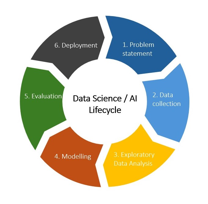
The six steps of DSL are listed below:
- Problem statement
- Data collection
- Exploratory data analysis
- Modelling
- Evaluation
- Deployment
Throughout the entire process, ethical considerations and professional conduct are essential and must be integrated into every step. Just as importantly, each step of the DSL is grounded in a deep understanding of the business context—without this, data science risks becoming disconnected from real-world impact.
In the chapters that follow, we illustrate how to apply the DSL to address practical business challenges. In addition to the six steps, we also emphasize communication and ethics as core components that must be embedded into the lifecycle.
Case Study: Pricing the Unpriceable
To make the DSL concrete before moving on, consider a real project completed through this course’s industry challenge program with a major Australian general insurer. The insurer’s name, exact figures, and identifying details have been changed or generalised. The data description, methodology, and results are otherwise faithful to the original project.
Monday Morning, Pricing Committee
Maria Alvarez, Head of Commercial Pricing at Wattle Insurance, had spent the weekend re-reading the same complaint for the third time. A regional broker had written in after losing a small business client: a suburban physiotherapy clinic, insured for building damage, had been quoted a premium nearly 40% higher than a competitor’s for what looked, on paper, like a near-identical risk. The broker’s question was blunt: “How can two similar businesses get such different prices from the same insurer, let alone from two different ones?”
It wasn’t the first time Maria had heard some version of this. Wattle’s small business (SME) building insurance book had grown quickly over the past few years, and with growth had come a widening set of occupations on the book, from cafes and hair salons to panel-beaters and cold-storage warehouses. Each was assigned an industry classification code, and each code was, in principle, priced according to its own risk. In practice, Maria knew the story was messier. She had a pricing committee meeting in three days and needed to decide what to bring to it.
Wattle Insurance is a mid-sized Australian general insurer with a long-standing personal lines business and a smaller, faster-growing commercial book. Small business building insurance, cover for the physical premises a business operates from, against fire, water damage, impact, storm, and similar perils, was one of the products driving that growth.
The Pricing Challenge
Australian businesses are classified using the Australian and New Zealand Standard Industrial Classification (ANZSIC), a four-level hierarchy running from broad Divisions (such as “Manufacturing”) down to granular Classes (such as “Meat Processing”). At the fine-grained end, there are hundreds to thousands of distinct occupation codes across the industries Wattle insured.
This granularity created a pricing problem. For any single occupation code, Wattle might have only a handful of policies and even fewer claims, nowhere near enough experience to estimate that occupation’s risk with any confidence. Pricing actuaries across the industry had two unappealing options: price each code individually, on very thin and noisy data, or lump codes together into broad, generic categories that ignored real differences in risk. Both approaches created the same downstream problem Maria was now facing: similar businesses priced inconsistently, and dissimilar businesses priced as if they were the same. Beyond the fairness and customer-experience issue, inconsistent pricing invited adverse selection, since brokers and customers would naturally steer towards whichever insurer had, often by accident, underpriced their particular occupation.
Maria had asked a small internal analytics team to see whether Wattle’s own claims data could support a better answer: a way of grouping occupations into hazard levels that was both statistically defensible and intuitive enough that an underwriter could explain it to a broker.
The Data
The team had access to five years of SME building claims data (2010-2015). Table 1 summarises the key fields. Beyond the claim itself (date, amount, and a peril field pre-classified into categories such as Fire, Water, Impact, and Accidental Damage), the data included the policyholder’s ANZSIC occupation code, tenure with the insurer, building construction details (roof, wall, and floor material), the presence of various fire protection features, the sum insured, and location.
One detail mattered more than it first appeared: the peril classification had been produced by a separate internal system that inferred the likely cause of loss from free-text loss descriptions and other claim details, using its own machine learning process. Nobody on the pricing team had built that system or knew exactly how it worked. It was simply handed to them as a given column.
| Field | Description |
|---|---|
totalIncurred |
Total gross incurred claim amount |
peril |
Vendor-classified cause of loss (Fire, Water, Impact, Accidental Damage, etc.) |
yearsInsured |
Tenure: years the policy has been held |
anzsic4_desc |
Occupation description (ANZSIC, 4-digit level) |
roofType / wallType / floorType |
Primary construction materials |
fireprotecAlarm, fireprotecMonitored, etc. |
Presence of various fire protection features |
BuildingSI |
Building sum insured |
stateRisk / postcodeRisk |
Location of the insured premises |
Building a Solution
Data preparation. Cleaning came first. Building material fields were missing for over 45% of records, too much to impute with any confidence, so the team coded “missing” as its own category rather than guessing. Records with negative claim amounts or implausible tenure values were removed. Postcode, too granular and sparse on its own, was regrouped into broader geographic regions.
Two patterns emerged that would shape everything that followed. Fire claims behaved differently from every other peril: rarer, but far more severe when they occurred. Buildings with wooden construction carried a noticeably higher average claim cost than other materials.
Grouping occupations. With hundreds of occupation codes and too little data to price most of them individually, the team turned to unsupervised learning. They applied k-means clustering to group occupations by similarity across four dimensions of claims experience: typical claim size, volatility, claim frequency, and the proportion of claims caused by fire. The result was nine ordinal hazard levels, from lowest to highest risk, each pooling together occupations that behaved similarly in the data regardless of what industry they were formally classified under. Service-oriented occupations tended to cluster toward the lower end. Retail and hospitality occupations tended toward the higher end.
Modelling claims cost. Using the new hazard levels alongside the other policy characteristics, the team built models to predict claims cost, fitting fire and non-fire perils separately given how differently they behaved. Three approaches were compared: a Generalised Linear Model (GLM), a Generalised Additive Model (GAM), and XGBoost. The team also built a fourth, more experimental model: a GLM with an XGBoost layer fitted to its residuals, intended to capture any structural pattern in the data the GLM had missed, while keeping the GLM’s coefficients interpretable for underwriters and regulators.
Results
Table 2 summarises model performance. XGBoost achieved the lowest prediction error, with the hybrid GLM-XGBoost model close behind, both outperforming the plain GLM by a modest margin. All four models agreed on something else too: building sum insured and regional risk consistently emerged as the two most important predictors of claims cost, more important than the occupation-based hazard level the team had spent most of their effort constructing.
| Model | RMSE | Interpretability |
|---|---|---|
| GLM | 73,707 | High |
| GLM + XGBoost residual layer (hybrid) | 71,660 | Medium |
| XGBoost | 71,333 | Low |
The team documented two open concerns of their own. First, their occupation clustering assumed that the mix of occupations in Wattle’s own portfolio matched national small-business statistics, since they had no access to Wattle’s full policy-level exposure data at the time, an assumption that might not hold, especially in geographic or industry segments where Wattle’s book was more or less concentrated than the national average. Second, they had used the vendor-supplied peril classification throughout without independently validating it. A separate task had asked them to try deriving peril categories from the raw loss descriptions themselves, but the team had not completed this in the time available.
The Decision Ahead
Maria now had a piece of analysis on her desk, and three days to decide what to do with it. A few questions kept circling:
- The hybrid model performed best, but it was harder to explain to underwriters, and harder to defend to a regulator, than a plain GLM. Was the accuracy gain worth the loss of transparency?
- Every model pointed to sum insured and region as the dominant drivers, with the carefully constructed occupation hazard levels adding comparatively little. Should Wattle still roll out the nine-level hazard grouping at all, or was the bigger opportunity somewhere else entirely?
- The clustering rested on an unverified assumption about Wattle’s own portfolio mix, and the whole exercise rested on a
perilclassification nobody on the team had built or fully validated. Were these acceptable risks to carry into a live pricing model, or did they need to be closed off first? - Underneath all of this was the original complaint from the broker. Would this new approach have actually changed the physiotherapy clinic’s premium, or was Maria about to present a technically impressive model that didn’t clearly fix the problem that started this?
Discussion Questions
- Walk through this case using the Data Science Lifecycle (Problem Statement, Data Collection, EDA, Modelling, Evaluation, Deployment). What was done well at each step, and where do you see gaps?
- The team’s four models disagreed on which technique fit best, but agreed on which variables mattered most. Which of these two pieces of information is more useful to Maria, and why?
- Should Maria recommend the interpretable GLM or the more accurate hybrid model? What would you want to know before answering that doesn’t appear in this case?
- The occupation-based hazard levels took most of the team’s effort but added comparatively little predictive power. Was building them a wasted exercise? What did the exercise accomplish even if the hazard levels themselves add limited lift?
- The clustering relied on an assumption about Wattle’s occupation mix that the team could not verify. How would you decide whether this assumption is safe enough to act on, versus a blocker that must be resolved first?
- The
perilfield came from a system the pricing team didn’t build and didn’t fully understand. What are the risks of building a pricing model on top of an input like this? What, if anything, should the team do about it before this goes into production? - Would this analysis have changed the outcome for the physiotherapy clinic from the opening scene? What would you need to check to answer that question?
Roadmap
The chapters are organised as follows:
Chapter 2 covers Step 1, focusing on how to ask the right question and frame it as a data science problem.
Chapter 3 addresses Steps 2 and 3, including data collection and exploratory data analysis.
Chapter 4 presents a range of modelling techniques, explaining when and how to apply them.
Chapter 5 introduces a systematic evaluation toolbox for data-driven decision-making, with a particular focus on applications in the insurance sector.
Chapter 6 explores effective communication strategies for engaging different stakeholders.
Chapter 7 introduces the Ethical Data Science (AI) Lifecycle (EDSL)—a framework for embedding ethical thinking across the entire DSL.